Building upon the success of MobileNetV1, Google released their latest network architecture, MobileNetV2. The new network architecture is built off of the original MobileNet model and has several improvements including increased throughput and improved accuracy. In this article, I will be introducing the inverted residual block (IRB) which is a key component of MobileNetV2.
Difference to other Networks
MobileNetV2 is the latest network training algorithm from Google, and it’s quite possibly one of the most important advances in deep learning since inception. The MobileNetV2 architecture is a modular network that allows for more flexibility and multiple layers of abstraction, making it easier to customize for specific tasks. Additionally, MobileNetV2 has been optimized for mobile devices and offers superior performance compared to other networks.
Heuristic of the (Inverted) residual block
First of all, let’s have a look at the figure. It already shows a clear distinction between the residual block and the inverted residual block.
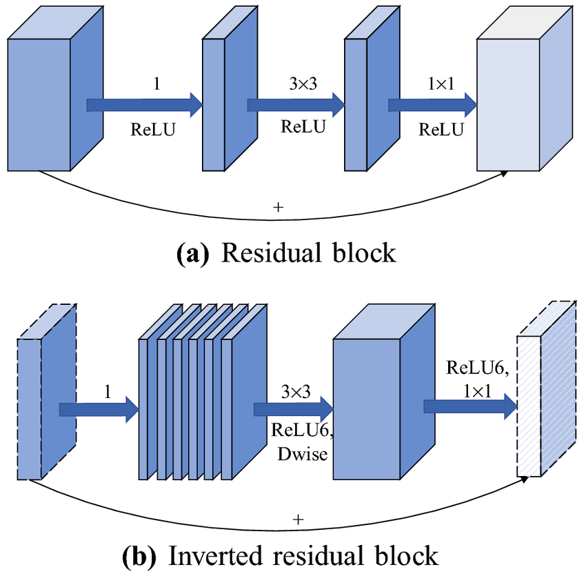
We can observe that an Initial residual block (a) follows the “wide- narrow- wide” strategy concerning the amount of channels. The input has multiple channels, which are lessened with a lightweight 1x1 convolution. In this manner, the next 3x3 convolution has a much smaller number of parameters. To impose inputs and outputs at the end of the number of channels is increased once again through another 1×1 convolution. In Keras it looked like this.
1
2
3
4
5
def residual_block(x, squeeze=16, expand=64):
  m = Conv2D(squeeze, (1,1), activation='relu')(x)
  m = Conv2D(squeeze, (3,3), activation='relu')(m)
  m = Conv2D(expand, (1,1), activation='relu')(m)
  return Add()([m, x])
MobileNetV2 goes about using a first-stage 1×1 convolution followed by a second-stage 3×3 convolution in the narrowing process. At the beginning of the narrowing process, MobileNetV2 uses a 1×1 convolution followed by the 3×3 convolution.
1
2
3
4
5
def inverted_residual_block(x, expand=64, squeeze=16):
  m = Conv2D(expand, (1,1), activation='relu')(x)
  m = DepthwiseConv2D((3,3), activation='relu')(m)
  m = Conv2D(squeeze, (1,1), activation='relu')(m)
  return Add()([m, x])
Advantages of the Inverted Residual Block
The Goal of any Neuronal network is to achieve a good performance. By the name of the MobileNet it is quite clear, that the performance is not only measured by accuracy or any similar metric. This model needs to perform a comparable accuarcy on an edge device like a mobile phone. Therefore the model size is quite important and with only around 20 MB it is extremely small. If you start comparing the runs of the two snippets above, you can see the inverted block has fewer parameters. This is one of the achievements compared to a ResNet model which is far bigger.
Further improvements
Empirically the performance of the current inverted residual block decreased by several percent and for this reason the authors came up with a linear bottleneck. This fancy solution prevents of destroying too much information and is easily implemented. We just remove in Tensorflow the ReLU activation function and we do have a linear activation.
1
2
3
4
5
def inverted_linear_residual_block(x, expand=64, squeeze=16):
  m = Conv2D(expand, (1,1), activation='relu')(x)
  m = DepthwiseConv2D((3,3),  activation='relu')(m)
  m = Conv2D(squeeze, (1,1))(m)
  return Add()([m, x])
Relu6 Activation function
Additionally the authors used ReLU6 instead of a ReLU, which limits the activation of activations to no more than a maximum of 6. The activation is straight until it is between 0 and 6.
1
2
3
4
5
def relu(x):
  return max(0, x)

def relu6(x):
  return min(max(0, x), 6)
This was introduced due to a fixed point precision in the MobileNetV1 Paper.
Final Inverted Residual Block
As the last part we need to add a BatchNormalization. Batch Normalization is a technique to normalize the activations in the Residual Network. It helps to solve problems of overfitting and it increases the performance.
1
2
3
4
5
6
7
8
9
10
def bottleneck_block(x, expand=64, squeeze=16):
  m = Conv2D(expand, (1,1))(x)
  m = BatchNormalization()(m)
  m = Activation('relu6')(m)
  m = DepthwiseConv2D((3,3))(m)
  m = BatchNormalization()(m)
  m = Activation('relu6')(m)
  m = Conv2D(squeeze, (1,1))(m)
  m = BatchNormalization()(m)
  return Add()([m, x])
Conclusion
MobileNetV2 is the latest iteration of Google’s state-of-the-art machine learning framework, and it offers a number of improvements over its predecessors. One of the most important changes is the introduction of inverted residual blocks, which allow for more accurate prediction by reducing the amount of noise in the data. I hope this article was helpful for you.
Many thanks to the authors of the articles:
The code blocks are from Paul-Louis Pröve blog post (towardsdatascience.com).
